Expanding mayavi 3D visualization toolkit
Before I could create functions for prisms and cylinders, I needed a way to easily rotate these objects in 3D space. I decided to implement a function to generate rotation matrices based on Euler angles. This would allow me to define a shape in a convenient coordinate system and then rotate it to the desired orientation. I created the following rotation_matrix function:
import numpy as np

def rotation_matrix(rx=0, ry=0, rz=0):
    """
    Calculates a rotation matrix given Euler angles (rx, ry, rz) in radians.

    Args:
        rx: Rotation angle around the x-axis.
        ry: Rotation angle around the y-axis.
        rz: Rotation angle around the z-axis.

    Returns:
        A 3x3 NumPy array representing the rotation matrix.
    """
    Rx = np.array([[1, 0, 0],
                   [0, np.cos(rx), -np.sin(rx)],
                   [0, np.sin(rx), np.cos(rx)]])
    Ry = np.array([[np.cos(ry), 0, np.sin(ry)],
                   [0, 1, 0],
                   [-np.sin(ry), 0, np.cos(ry)]])
    Rz = np.array([[np.cos(rz), -np.sin(rz), 0],
                   [np.sin(rz), np.cos(rz), 0],
                   [0, 0, 1]])
    return Rz @ Ry @ Rx
This function takes three arguments: rx, ry, and rz, representing the rotation angles around the x, y, and z axes, respectively, in radians. It then constructs the individual rotation matrices for each axis and combines them using matrix multiplication to produce the final rotation matrix. I chose the ZYX convention for the Euler angles. With this function in place, I had a fundamental tool for manipulating the orientation of my 3D primitives. This was a crucial step before creating the functions for prisms and cylinders, as it allowed me to generate these shapes in a standard orientation and then rotate them as needed.
Creating prisms
Following the development of the rotation matrix function, I implemented the plot_prism function to generate and visualize prisms in Mayavi. This function offers control over various aspects of the prism’s appearance and behavior. Here’s the function signature and a description of its parameters:
def plot_prism(mlab, center, dim_1, dim_2, height, color=c.b, opacity=1.0,
               plot_base=True, base_color=c.r, base_opacity=None,
               edge_color=None, edge_width=1.0, R=np.eye(3)):
    """
    Plots a prism

    Args:
        mlab: The Mayavi mlab object to use for plotting.
        center: The base coordinates of the prism (x, y, z) as a 3-tuple.
        dim_1: The length of the prism along one horizontal axis.
        dim_2: The length of the prism along the other horizontal axis.
        height: The height of the prism.
        color: The color of the prism (default: blue).
        opacity: The transparency of the prism (default: 1, fully opaque).
        edge_color: The color of the edge lines (default: None).
        edge_width: The width of the edge lines (default: 1.0).
        plot_base: Whether to plot the top and bottom bases (default: True).
        base_color: The color of the top and bottom base (default: red).
        base_opacity: The transparency of the bases (default: same as opacity).
        R: The rotation matrix for the prism (default: no rotation).
    """
The center argument, a tuple of (x, y, z) coordinates, defines the base location of the prism in 3D space. The dim_1 and dim_2 parameters specify the prism’s dimensions along its two horizontal axes, defining its width and depth. The height parameter determines the prism’s vertical extent.
The color argument sets the color of the prism’s main body, accepting an RGB tuple; I use a custom color module c, but standard RGB tuples like (1, 0, 0) for red are also valid. The opacity value controls the prism’s transparency, with 1 being fully opaque and values between 0 and 1 allowing for partial transparency.
The plot_base boolean flag determines whether the top and bottom faces of the prism are rendered; it defaults to True. The base_color argument allows for a distinct color for these bases, defaulting to red. The base_opacity parameter controls the transparency of the bases, defaulting to the same value as the main body’s opacity if not explicitly set.
The R argument accepts a 3x3 rotation matrix, defaulting to the identity matrix for no rotation; this is where my previously defined rotation_matrix function is used. The edge_color argument, when provided as a color tuple, enables the visualization of the prism’s edges. Finally, the edge_width parameter controls the thickness of these edge lines, defaulting to 1.0.
    # ... (Inside the function)
    # Apply rotation
    rotated_vertices = np.dot(vertices - center, R.T) + center

    # ... (Rest of the implementation)
This snippet shows how the rotation matrix R is applied to the prism’s vertices. This is one of the step for orienting the prism in 3D space.
Overall, this plot_prism function offers a flexible tool for creating and customizing prisms within your Mayavi visualizations. The various options allow you to tailor the appearance and orientation of these shapes to precisely match your engineering needs. I found this function very useful in my own projects for visualizing various mechanical components.
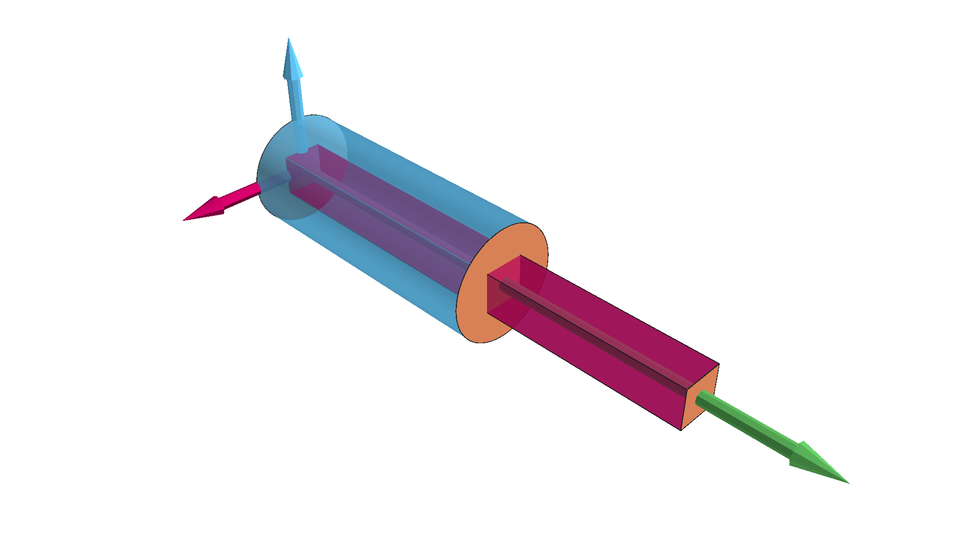
Creating cylinders
I developed plot_cylinder to generate and visualize cylinders in Mayavi. This function offers control over various aspects of the cylinder’s appearance and behavior. Here’s the function signature and a description of its parameters:
def plot_cylinder(mlab, center, radius, height, color=c.b, opacity=1.0,
                  plot_base=True, base_color=c.r, base_opacity=None,
                  edge_color=None, edge_width=1.0, R=np.eye(3)):
    """
    Plots a cylinder

    Args:
        mlab: The Mayavi mlab object to use for plotting.
        center: The center coordinates of the cylinder (x, y, z) as a 3-tuple.
        radius: The radius of the cylinder base.
        height: The height of the cylinder.
        color: The color of the cylinder body (default: blue).
        opacity: The transparency of the cylinder (default: 1, fully opaque).
        plot_base: Plot the base and top circles (default: True).
        base_color: The color of the cylinder head circles (default: red).
        base_opacity: The transparency of the base (default: 1, fully opaque).
        edge_color: The color of the edge lines (default: None).
        edge_width: The width of the edge lines (default: 1/1000).
        R: The rotation matrix for the cylinder (default: identity matrix).
    """
The center argument, provided as a tuple of (x, y, z) coordinates, defines the center point of the cylinder in 3D space. The radius parameter specifies the radius of the cylinder’s circular base. The height parameter determines the cylinder’s vertical extent.
The color argument sets the color of the cylinder’s main body, accepting an RGB tuple; I use a custom color module c, but standard RGB tuples like (1, 0, 0) for red are also valid. The opacity value controls the cylinder’s transparency, with 1 representing fully opaque and values between 0 and 1 allowing for partial transparency.
The plot_base boolean flag determines whether the top and bottom circular faces of the cylinder are rendered; it defaults to True. The base_color argument allows for a distinct color for these circular bases, defaulting to red. The base_opacity parameter controls the transparency of the bases, defaulting to the same value as the main body’s opacity if not explicitly set.
The R argument accepts a 3x3 rotation matrix, defaulting to the identity matrix for no rotation; this is where my previously defined rotation_matrix function is used. It enables you to define the cylinder’s initial orientation in 3D space. The edge_color argument, when provided as a color tuple, enables the visualization of the cylinder’s edges. Finally, the edge_width parameter controls the thickness of these edge lines, defaulting to 1.0.
Inside the function, the cylinder body is created by defining a grid of points using np.linspace for the angle (theta) and z-coordinates (height). These points are then converted to Cartesian coordinates (X, Y, Z) based on the radius and angle values. The points are reshaped to match the grid dimensions and then rotated using the provided rotation matrix R. Finally, mlab.mesh is used to render the cylinder body with the specified color and opacity.
The code then checks the plot_base flag. If it is True, the code iterates over the top (z-offset equals height) and bottom (z-offset equals 0) of the cylinder. Similar to the body creation, a grid of points is defined for each circular base using np.linspace for the angle and radius. These points are converted to Cartesian coordinates and rotated using R. mlab.mesh is used to render these circular faces with the base_color and specified base_opacity.
If an edge_color is provided, the function creates the edges of the cylinder. It does this by creating points along the top and bottom circles of the cylinder and then using mlab.plot3d to draw lines between these points. The rotation matrix is also applied to these edge points. This provides a clear outline of the cylinder. This function provides a versatile way to create and customize cylinders within Mayavi visualizations.
Conclusion
In this blog post, I expanded my Mayavi 3D visualization toolkit by implementing functions for creating two essential geometric primitives: prisms and cylinders. Building upon the previously created rotation_matrix function, I developed plot_prism and plot_cylinder to offer precise control over the appearance, dimensions, and orientation of these shapes.
The plot_prism function allows for customization of the prism’s dimensions, color, opacity, the presence and appearance of its bases, and its rotation in 3D space. Similarly, the plot_cylinder function provides control over the cylinder’s radius, height, color, opacity, the presence and appearance of its circular faces, and its rotation. These functions significantly enhance my ability to visualize complex mechanical designs and simulations within my engineering workflow. By providing these reusable building blocks, I aim to streamline my visualization process and offer helpful tools for other engineers working with Mayavi. In future posts, I plan to continue expanding this toolkit with additional primitives and more advanced visualization techniques.