Enhancing mayavi visualizations with matplotlib textures
In this blog post, I describe my method for improving text rendering within Mayavi visualizations. I found Mayavi’s built-in text rendering to be limited, especially concerning LaTeX support and font choices. To address this, I developed a hybrid solution using Matplotlib to create text as PNG images, which are then imported as textures into Mayavi.
The render_text function handles this process. Its purpose is to create a texture with LaTeX-rendered text and apply it to a 3D surface within Mayavi. The function takes several arguments. The text argument is the LaTeX code for the text to be rendered. The optional size argument sets the font size; if not provided, it defaults to 30. The color argument sets the text color. The position argument, a tuple of (x, y, z) coordinates, sets the text’s position in 3D space. The orientation argument, also a tuple, sets the text’s orientation, typically matching the camera view; it defaults to a common orientation for 3D scenes (azimuth = 45°, elevation arctan(√2)). The scale argument, defaulting to (1, 1, 1), scales the texture. The image_size argument sets the size of the generated image.
def render_text(mlab, text, size=None, color=(0, 0, 0), position=(0, 0, 0),
                orientation=(0, 54.735610317245346, 45), scale=np.ones(3),
                image_size=(512, 512)):
    """
    Creates a texture with LaTeX-rendered text, applies it to a 3D surface in the Mayavi context.

    Args:
        text (str): LaTeX text to render.
        size (int): Font size for the text.
        color (str): Text color.
        position (tuple): (x, y, z) position of the text in the 3D space.
        orientation (tuple): orientation in the space (should be the same as
                            camera, (default: azimuth = 45°, elevation arctan(√2))
        scale (tuple): scaling factor to apply (default: 1)
        image_size (tuple): Size of the generated image (width, height).
    """
    plt.rcParams['text.latex.preamble'] = r"\usepackage{bm} " \
                                          r"\usepackage{amsmath} \usepackage{helvet}"
    plt.rcParams.update({
        "text.usetex": True, "font.family": "Helvetica",
        "font.sans-serif": "Helvetica"})

    fig, ax = plt.subplots(figsize=(image_size[0] / 300, image_size[1] / 300), dpi=300)
    ax.axis('off')
    fig.patch.set_alpha(0)
    ax.patch.set_alpha(0)
    if size is None:
        size = 30
    ax.text(0.5, 0.5, text, fontsize=size, color='k', ha='center',
            va='center', transform=ax.transAxes)

    temp_file = "temp_texture.png"
    fig.savefig(temp_file, dpi=300, transparent=True)
    plt.close(fig)

    with Image.open(temp_file) as img:
        img_array = np.array(img.getdata(), np.uint8)
        img_array.shape = (img.size[1], img.size[0], 4)

    if len(color) == 3:
        color = (255 * color[0], 255 * color[1], 255 * color[2], 255)
    mask = img_array[:, :, 3] > 0
    img_array[mask] = color
    my_lut = img_array.reshape(-1, 4)

    my_lut_lookup_array = np.arange(img_array.shape[0] * img_array.shape[1])
    my_lut_lookup_array = my_lut_lookup_array.reshape(img_array.shape[:2])

    im = mlab.imshow(my_lut_lookup_array, colormap='binary')

    im.module_manager.scalar_lut_manager.lut.table = my_lut
    im.actor.orientation = orientation
    im.actor.position = position
    if isinstance(scale, (float, int)):
        scale = np.ones(3) * scale
    im.actor.scale = scale / 500
    os.remove(temp_file)
The function begins by configuring Matplotlib for LaTeX rendering, including necessary packages like bm and amsmath and setting the font to Helvetica. A transparent Matplotlib figure and axes are created for rendering the text. The figsize is calculated based on the desired image_size and a DPI of 300. The axes and figure backgrounds are set to transparent. The LaTeX-formatted text is then added to the Matplotlib axes, centered both horizontally and vertically. The figure is saved as a temporary transparent PNG file named "temp_texture.png", and the Matplotlib figure is closed to free memory.
The saved PNG image is loaded using PIL (Pillow) and converted to a NumPy array. The array is reshaped to have RGBA channels. If a 3-tuple RGB color is provided, it’s converted to RGBA. A mask is created to select only the non-transparent pixels (the text), and the desired color is applied to these pixels. The image array is flattened to create a lookup table (LUT) for Mayavi’s imshow function. A lookup array for imshow is created, which is a 2D array of indices corresponding to the LUT. The image is displayed in Mayavi using imshow, creating the textured plane.
The lookup table of the image object is updated with the color data from the PNG. The textured plane (text) is positioned and oriented in the 3D scene using the provided position and orientation arguments. The text is scaled, with an empirical adjustment of dividing by 500 for reasonable scaling. Finally, the temporary PNG file is removed. This function offers a way to incorporate high-quality, LaTeX-rendered text into Mayavi visualizations, overcoming its native limitations.
Conclusion
This hybrid approach, using Matplotlib for text rendering and importing the result as a texture into Mayavi, effectively overcomes Mayavi’s limitations with LaTeX support and font selection. By generating text as PNG images, I gain complete control over font styling, LaTeX formatting, and image resolution. This method provides a flexible and powerful way to add rich text annotations to my 3D visualizations.
For example, I can render complex mathematical equations directly within my Mayavi scenes. Consider the following code snippet that renders two well-known physics equations:
render_text(mlab, r'$ \mathbf F = m \cdot \mathbf a '
                    r'= m \frac{\mathrm d \mathbf v}{\mathrm dt} '
                    r'= m \frac{\mathrm d^2 \mathbf r}{\mathrm dt^2}$',
            position=(0.0, 0.0, 1.3), scale=1.0, image_size=(1600, 300),
            color=c.r)
render_text(mlab, r'E = m \, c^2',
            position=(0.4, 0.6, 0), orientation=(0, 0, 0),
            scale=1.0, image_size=(1600, 300),
            color=c.b)
This code renders Newton’s second law of motion and Einstein’s mass-energy equivalence. The image_size parameter allows me to control the resolution of the generated text, ensuring clear and readable labels even at different zoom levels. The position, orientation, and scale parameters allow me to precisely place and size the text within the 3D scene. The use of raw strings (r’…’) is essential for correctly interpreting LaTeX code in Python.
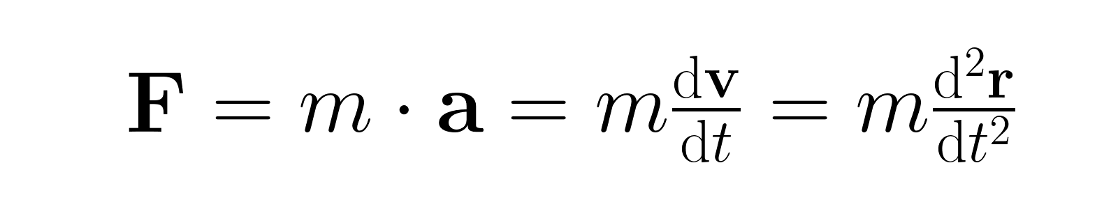
This link shows the texture generated for Newton’s second law. Notice the high quality of the rendered LaTeX.

This link displays the texture generated for Einstein’s famous equation. The different positioning and color demonstrate the flexibility of the render_text function.
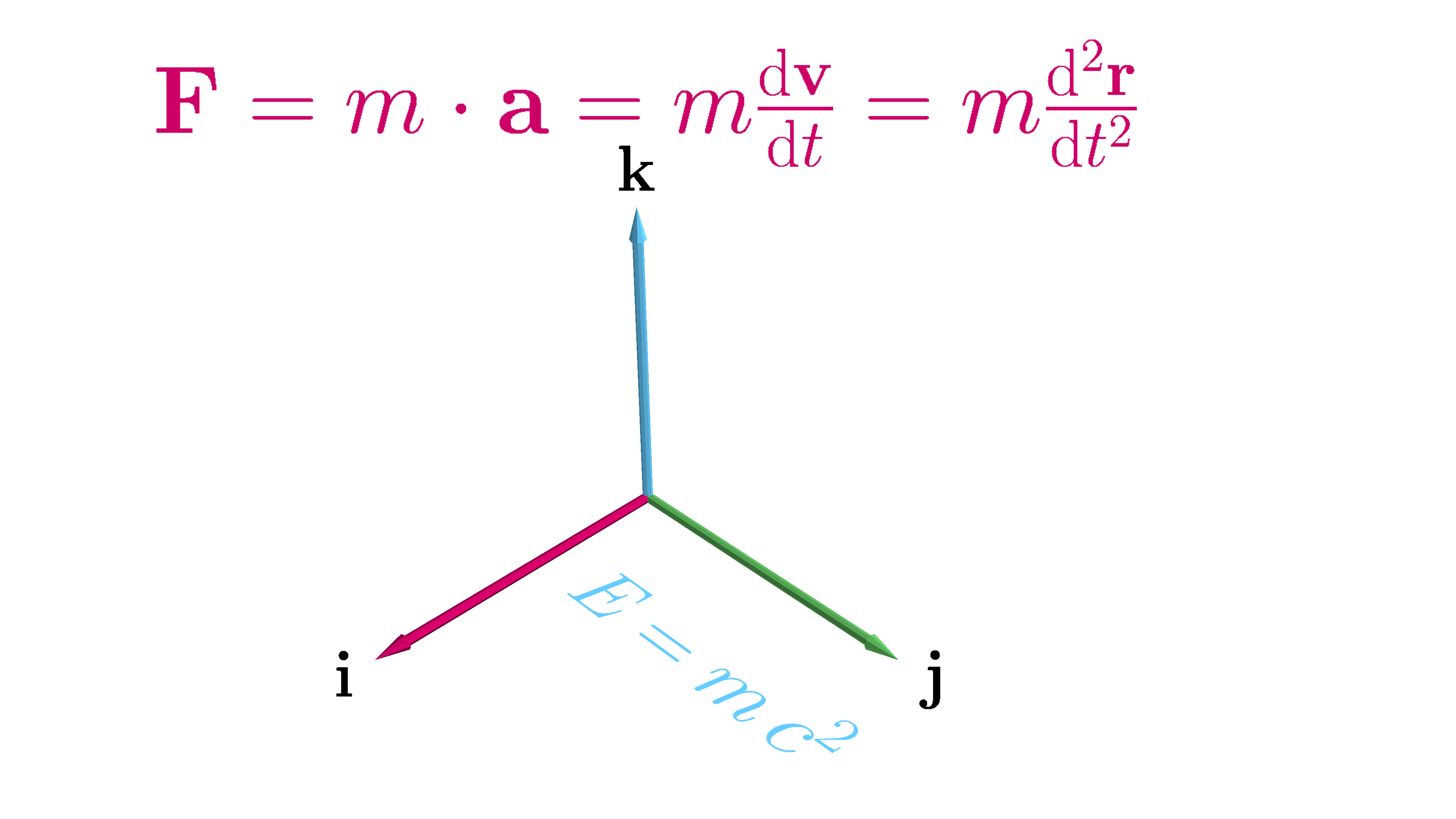
This link shows the final result within the Mayavi scene, with both equations correctly positioned and rendered as textures. This hybrid approach has become an essential part of my Mayavi workflow, allowing me to create informative and visually appealing 3D visualizations.