Lagrangian mechanics example: rectilinear motion
After deriving Lagrange’s equations, it is helpful to see them in action. I will start with the simplest non-trivial case: the motion of a particle along a straight line under a conservative force.
Consider a particle of mass m restricted to move along the x-axis. Its configuration is completely described by its position x. Therefore, there is only one degree of freedom, and the generalized coordinate is simply q_1 = x.
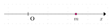
The velocity of the particle is \dot x. The kinetic energy T is:
T = \frac{1}{2} m \dot x^2
Assume the particle is subject to a conservative force derivable from a potential energy function V(x). The Lagrangian L is defined as \mathcal L = T - V:
\mathcal L = \frac{1}{2} m \dot x^2 - V(x)
Applying Lagrange’s equation
For a conservative system with one generalized coordinate x, Lagrange’s equation is:
\frac{\mathrm d}{\mathrm d t} \left( \frac{\partial \mathcal L}{\partial \dot x} \right) - \frac{\partial \mathcal L}{\partial x} = 0
I need to compute the partial derivatives of L with respect to \dot x and x.
First, the derivative with respect to the generalized velocity \dot x:
\frac{\partial \mathcal L}{\partial \dot x} = \frac{\partial}{\partial \dot x} \left( \frac{1}{2} m \dot x^2 - V(x) \right)
Since V(x) does not depend on \dot x, its partial derivative with respect to \dot x is zero. Thus:
\frac{\partial \mathcal L}{\partial \dot x} = \frac{1}{2} m (2 \dot x) = m \dot x
Next, the derivative with respect to the generalized coordinate x:
\frac{\partial \mathcal L}{\partial x} = \frac{\partial}{\partial x} \left( \frac{1}{2} m \dot x^2 - V(x) \right)
The kinetic energy term \frac{1}{2} m \dot x^2 does not explicitly depend on x (only on \dot x), so its partial derivative with respect to x is zero. Therefore:
\frac{\partial \mathcal L}{\partial x} = -\frac{\partial V}{\partial x}
Recovering Newton’s second law
Now, I substitute these partial derivatives back into Lagrange’s equation:
\frac{\mathrm d}{\mathrm d t} (m \dot x) - \left( -\frac{\partial V}{\partial x} \right) = 0
Performing the time derivative:
m \ddot x + \frac{\partial V}{\partial x} = 0
Recognizing that the force F_x in one dimension derived from a potential V(x) is F_x = -\frac{\partial V}{\partial x}, I can rewrite the equation as:
m \ddot x - F_x = 0
or
m \ddot x = F_x
This is exactly Newton’s second law for motion in one dimension. This example shows how the Lagrangian formalism, starting from scalar quantities (kinetic and potential energy), reproduces the familiar equations of motion derived from vector mechanics. While seemingly more elaborate for this simple case, its power becomes evident in more complex systems with multiple coordinates and constraints.
For more insights into this topic, you can find the details here.