Lagrangian mechanics example: the pendulum
Following the rectilinear motion example, I now tackle a slightly more complex system using the Lagrangian approach: the simple mathematical pendulum. This problem involves motion constrained to a circular path in a gravitational field.
The system consists of a point mass m attached to one end of a rigid, massless rod of length r. The other end of the rod is fixed at a pivot point O. The pendulum swings in a vertical plane under the influence of uniform gravity g.
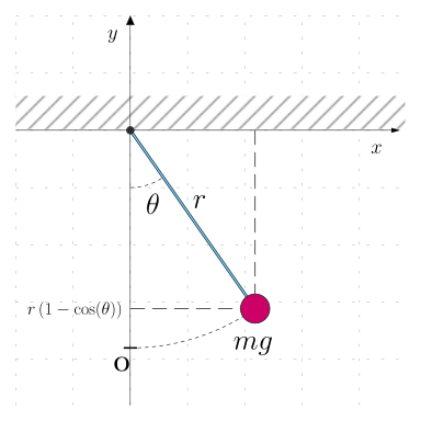
The position of the mass m is uniquely determined by the angle \theta the rod makes with the downward vertical direction. Therefore, the system has only one degree of freedom, and I choose \theta as the generalized coordinate (q_1 = \theta).
Kinetic and Potential Energy
First, I determine the kinetic energy T. The mass moves along a circular arc. Its speed v is the tangential speed, given by v = r |\dot\theta|, where \dot\theta is the angular velocity. The kinetic energy is:
T = \frac{1}{2} m v^2 = \frac{1}{2} m (r \dot\theta)^2 = \frac{1}{2} m r^2 \dot\theta^2
Next, I determine the potential energy V. I set the reference level for gravitational potential energy (V=0) at the lowest point of the pendulum’s swing (where \theta=0). Relative to this level, the height h of the mass at an angle \theta is h = r - r \cos \theta. The potential energy is thus:
V = mgh = mgr(1 - \cos \theta)
The Lagrangian
The Lagrangian L is defined as \mathcal L = T - V:
\mathcal L = \frac{1}{2} m r^2 \dot\theta^2 - mgr(1 - \cos \theta)
Notice that the term -mgr in V (and thus in L) is a constant. Since Lagrange’s equations involve derivatives of L, constant terms do not affect the final equations of motion. I can therefore work with a simplified Lagrangian by dropping this constant term, which is equivalent to choosing the potential energy zero level at the pivot point (h = -r \cos \theta):
\mathcal L = \frac{1}{2} m r^2 \dot\theta^2 + mgr \cos \theta
I will use this form.
Applying Lagrange’s equation
For the generalized coordinate \theta, Lagrange’s equation is:
\frac{\mathrm d}{\mathrm d t} \left( \frac{\partial \mathcal L}{\partial \dot\theta} \right) - \frac{\partial \mathcal L}{\partial \theta} = 0
I calculate the necessary partial derivatives using L = \frac{1}{2} m r^2 \dot\theta^2 + mgr \cos \theta.
The derivative with respect to the generalized velocity \dot\theta:
\frac{\partial \mathcal L}{\partial \dot\theta} = \frac{\partial}{\partial \dot\theta} \left( \frac{1}{2} m r^2 \dot\theta^2 + mgr \cos \theta \right) = m r^2 \dot\theta
This term corresponds to the angular momentum of the mass about the pivot.
The derivative with respect to the generalized coordinate \theta:
\frac{\partial \mathcal L}{\partial \theta} = \frac{\partial}{\partial \theta} \left( \frac{1}{2} m r^2 \dot\theta^2 + mgr \cos \theta \right) = -mgr \sin \theta
This term is related to the gravitational torque acting on the mass.
Equation of motion
Substituting these derivatives into Lagrange’s equation:
\frac{\mathrm d}{\mathrm d t} (m r^2 \dot\theta) - (-mgr \sin \theta) = 0
Since m and r are constants, the time derivative is:
m r^2 \ddot\theta + mgr \sin \theta = 0
Finally, dividing by the constant factor mr^2 (assuming m \neq 0, r \neq 0), I obtain the equation of motion for the simple pendulum:
\ddot\theta + \frac{g}{r} \sin \theta = 0
This is the standard nonlinear second-order ordinary differential equation describing the angular motion of the simple pendulum. This derivation illustrates the power and elegance of the Lagrangian method: by simply writing down the scalar kinetic and potential energies in terms of the chosen generalized coordinate, the application of Lagrange’s equation directly yields the correct equation of motion, bypassing the need to analyze vector forces, tensions, and constraint forces explicitly.
For more insights into this topic, you can find the details here.